Data, data everywhere, and not a drop to think

Data mining is and is not data analysis

Data, data everywhere and not a .... to use

Source: Delaine Hampton, presented at Marketing Science Conference (June 2004).

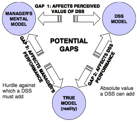
Source: Kayande et al. (2009)

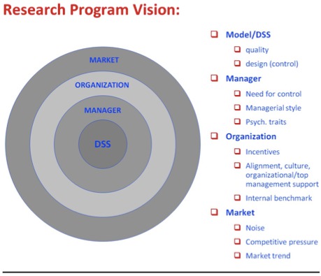
Source: Lilien (2011)

the distinct segments or groups must satisfy at least the following criteria (cf. Leeflang 1994, p. 41, and Wedel 1990, p. 17):

• the size and composition of the selected group must be known.
• it must be possible to reach the selected group effectively in a communicative manner.
• the selected group should be economically large enough for the development of a promotional campaign.

Since a mailing list contains at least names and addresses, each individual can be reached by mail. The last criterion is met when the number of individuals in the group that should receive a mailing is sufficiently large. This number implicitly depends on the revenues to a positive reply, the costs of a single mailing piece and the fixed costs.

Hence, a mailing list offers an organization a perfect possibility for effective segmentation, which coincides with target selection here.

We distinguish three classes of objectives for the consumer market (e.g.Roberts and Berger 1989, p. 9):

1. The accomplishment of the sale of a product or service. This is the most frequently used objective.

2. The generation of leads, denoting the request of an individual for additional information about the subject. In the next stage, an organization may try to convert these leads into sales. Expensive or complex products, like insurance policies, are often sold by this two-stage process. For a successful campaign the organization should not only focus on generating leads but also in the conversions of these leads.

3. The maintenance of customer relationships. The mailing under consideration does not have the purpose to sell the product or to generate leads, but to strengthen the relation (e.g. a newsletter of an insurance company which is sent to all the policy holders).

Selection variables, often called segmentation variables in the direct marketing literature, are of course a crucial element for target selection. If the available variables do not have any explanatory or discriminatory power to distinguish respondents from non respondents, segmentation is not very useful.

Four basic categories of selection variables can be distinguished (Roberts and Berger 1989, p. 106):

(1) geographic variables, (2) demographic variables, (3) psychographic or lifestyle variables and (4) behavioural variables.  

Within direct marketing the behavioural variables, in particular variables related to the individuals’ purchase history, are considered the most important.

They include the recency of the last purchase, the frequency of purchases and the monetary amount spent on the purchases (e.g. Roberts and Berger 1989, p. 106); the so-called RFM-variables.

Recency includes the number of consecutive mailings without response and the time period since the last order.

Frequency measures include the number of purchases made in a certain time period.

Monetary value measures include the amount of money spent during a certain period.

It is clear that this kind of information solely relates to individuals previously mailed. A database with this type of customer information is called the internal list(e.g. Bickert 1992). This list often also includes individuals who have never bought a product but only made an inquiry or to whom a mailing has been directed.

These lists contain geographical variables (region, degree of urbanization), demographic variables (age, sex, family size) and lifestyle characteristics (habits, leisure interests).

External lists may be put together for direct marketing support or for other reasons (e.g. telephone directories). It is important to realize that external lists can be used as additional information to the internal list but may also be the only source of information. The latter is often the case when the mailing is directed to acquire new customers. External lists can be rented from commercial companies. In the United States these lists are offered by, among others, R.L. Polk, National Demographics and Lifestyles and Database America.

 In the Netherlands lists can be rented from Geo-Markt profiel, Mosaïc and recently from Calyx (in cooperation with Centrum voor Consumenten Informatie). A comprehensive discussion on the use of commercial databases can be found in Lix et al. (1995).

For selection one should decide whether a step-wise procedure should be used to select the explanatory variables or a so-called forced entry, i.e. including all the variables (chosen a priori).

Transformation of variables is employed, for instance, in the following two situations:

(1) recode a categorical variable that has (too) many categories;

(2) incorporate a continuously measured variable in a flexible, i.e. non-linear, way. A straightforward way to do so is by dividing this variable into a number of categories and using a dummy variable for each category; this is often called binning(Lix and Berger 1995).

Generally, selection takes place on the basis of some measure of response. For direct mail, three kinds of responses can be distinguished, depending on the offer submitted in the mailing.

• The first kind concerns mailings with fixed revenues (given a positive reply), such as subscriber mailings of a magazine, membership mailings and single-shot mailings offering just one product, for example a book.
• A second kind concerns mailings where the response is the number of units ordered, e.g. the number of compact discs ordered by direct mail selling or the subscription time (a quarter of a year, half a year, a full year) when a magazine is offered through direct mail.
• Third, there are mailings with a response that can take on all positive values. This may involve total revenues in purchases from a catalog retailer, or the monetary amount donated to a charitable foundation raising funds by mail.

Nearly all the selection techniques that have been proposed deal with the case of fixed revenues to a positive reply.

We start the overview with the RFM-model, which is the pioneering method of list segmentation.

Subsequently, we discuss two techniques, the contingency table and CHAID, which are sometimes classified as clustering-like methods (Cryer et al. 1989), since the analysis generates clusters as output.

Then we present several specifications that focus on the binary choice, like probit and logit models, discriminant analysis, the beta-logistic model and latent class analysis.

Finally, we present the neural network approach, which is an alternative to conventional statistical methods. We assume that a test mailing is sent to a relatively small sample of individuals of the mailing list. Then, one of the techniques is employed to link the (non)response to the segmentation variables. Next, the technique is used to select the most promising targets on the mailing list.

Traditionally, the so-called RFM-model is most frequently used for target selection. As its name suggests, it is solely based on the RFM variables. Each RFM-variable is split into a number of categories, which are chosen by the researcher. To each of those categories a score is assigned, which is the difference between the average response rate and the observed response rate in that category. For an individual we obtain a score by adding his category scores. This enables us to rank the individuals on the mailing list. The advantage of this method is its simplicity. The drawback is that the model does not account for multicollinearity unless the RFM-variables are mutually independent. Furthermore, it is not clear which individual should receive a mailing. Bauer (1988) extended this method by using the RFM-model in a functional relationship in which the unknown parameters are determined a priori.

The simplest method of modelling response is by a contingency table. It is a two- or more dimensional matrix of which the dimensions are determined by the number of variables involved. Each of these variables is divided into a number of categories. Each specific combination of categories, i.e. one category for each variable, defines a cell.

For target selection contingency tables can be used as follows:

• the researcher chooses the variables to be taken into account.
• If a variable is continuous, it has to be categorized.
• On the basis of these categories the individuals are scanned and assigned to a cell.
• In each cell the response rate is computed, which is used to decide whether the individuals belonging to that cell should be selected.

It is a nonparametric method which can be classified as non-criterion based (Magidson 1994), denoting that the clusters, i.e. cells, are not explicitly derived on the basis of a dependent variable. This implies that the continuous variables, or variables with too many categories that have to be recategorized, are categorized in a rather ad-hoc manner. The major drawback of this method is that it becomes very disorderly in the case ofmany variables, with the risk of having not enough observations per cell, which is the curse of dimensionality. It can, however, be very useful for a first data analysis in order to choose selection variables for further analysis.

Automatic interaction detection (AID), the predecessor of CHAID, is based on a stepwise analysis-of-variance procedure (Sonquist 1970). The dependent variable is interval-scaled and the independent variables are categorical.

AID consists of the following steps:

(a) for every independent variable the optimal binary split is determined in such a way that the within-group variance of the dependent variable is minimal. That is, AID merges the categories of an independent variable which are, more or less, homogeneous with respect to the dependent variable. For each independent variable this results in an optimal binary split;

(b) the variable that generates the lowest within-group variance is used to subdivide the dependent variable in accordance with its optimal binary split;

(c) given this binary split, two groups are constructed. Each group is analyzed in the same manner as defined by (a) and (b).

This process continues until some stopping criterion is satisfied. This criterion can be either a number of segments or number of individuals in a segment.

The result is a treelike group of segments; it is a so-called tree-building method. The individuals that belong to a segment with a sufficiently high response rate should be selected.

The CHAID, developed by Kass (1980), improves the AID in several respects. CHAID merges categories of an independent variable that are homogeneous with respect to the dependent variable, but does not merge the other categories.

The result of this merging process, unlike AID, is not necessarily a dichotomy. Hence, steps (a) and (b) may result in more than two subgroups. On the other hand, also in contrast with AID, only those independent variables are eligible to be split into subgroups for which the subgroups differ significantly from each other; the significance is based on a _2-statistic. This explicitly defines a stopping rule. Note that it is a nonparametric technique since it does not impose a functional form for the relation between the dependent and independent variables. In contrast with cross-tabulation, it may be classified as criterion-based since the splits are derived on the basis of a dependent variable. The main advantage of (CH)AID is that the output is easy to understand and therefore easy to communicate to the management.

In practice it is often seen as a useful exploratory data analysis technique, in particular to discover interaction effects among variables, of which output may be used as input for other techniques with more predictive power (Shepard 1995).Magidson (1994) provides an extensive examination on CHAID.

A closely related technique is the so-called classification and regression trees(CART), which was developed by Breiman et al. (1984). The result of this technique is also a treelike group of segments.

In contrast with CHAID, the independent variables may be categorical and continuous. The splits are based on some homogeneity measure between the segments formed. Like CHAID, it is a useful method for explorative data analysis and also easy to communicate. A comprehensive discussion on CART can be found in Haughton and Oulabi (1993) and Thrasher (1991).

Un bonne partie la littérature sur l’apprentissage machine, est préocuupé par les variables logique et par des decisions correctes. Le résultat d’un arbre est un partition de l’espace X des observations possibles. Dans les problème logique on suppose qu’il y a une partition de l’espace X qui va classifier correctement toutes les observations, et l’objectif est de trouver

Du faite

Regression analysis with a dichotomous dependent variable (response/nonresponse) is called a linear probability model. The predicted value can be interpreted as the response probability. This probability is assumed to depend on a number of characteristics of the individuals receiving the mailing. That is

 where yi is a random variable that takes the value one if the ith individual responds and zero otherwise, xi is a vector of characteristics of i, i.e. RFM-variables, geographic and demographic variables etc.; ui is a random disturbance, and _ is an unknown parameter. The unknown parameters can be estimated by ordinary least squares (OLS). On the basis of the estimated response probability the potential targets can be ranked in order to make a selection.

This model has several readily apparent problems (Judge et al. 1985, p. 757). For example, the use of OLS will lead to inefficient estimates and imprecise predictions. The relation is very sensitive to the values taken by the explanatory variables, and the estimated response probability can lie outside the [0; 1]-interval.

An alternative way to handle discrete response data is by the probit or logit model. These models overcome the disadvantages of the linear probability model. Probit and logit models assume that there is a latent variable,  , which measures the inclination to respond, which depends on a vector of individual characteristics. That is,

 As we cannot observe the inclination but only whether or not i responded, we define the dependent variable which we observe, as

(2.2)

The probit model assumes that the distribution of ui is normal and the logit model assumes that ui is logistic.With these fully parametric specifications, the model can easily be estimated by maximum likelihood (ML). The individuals for which the predicted response probabilities is sufficiently high are selected for the direct mailing campaign. In chapters 3, 4 and 5 we elaborate on the probit model in more detail. Bult andWansbeek (1995) argue that the selection procedure rests heavily upon the functional formof the disturbance, which could cause inconsistent estimates and would consequently lead to a suboptimal selection rule. Therefore, they use the semiparametric method developed by Cosslett (1983) to estimate the parameters. This method not only maximizes the likelihood function over the parameter space, _, but also over the space which contains all the distribution functions. Of course, other semiparametric estimators of the binary choice model, e.g. Klein and Spady (1993), could be used as well.

Rao and Steckel (1995) consider a beta-logistic model for the binary choice to allow for heterogeneity. Let pi be the probability of obtaining a response from i. The heterogeneity in pi is assumed to be captured by a beta distribution with parameters ai and bi. That is,

 where B.ai ; bi / is the beta function defined by

 Rao and Steckel favor this distribution mainly because it is flexible so that it can take on a variety of shapes (flat, unimodel, J-shaped), depending on its parameters. The mean, ai=.ai C bi / could serve as the response probability for individual i. The variation in the response probability among similar individuals is thus described by the beta distribution. The parameters ai and bi are modeled as exponential functions of the selection variables (Heckman and Willis 1977), i.e. ai D exp._01 xi / and bi D exp._02 xi /. Loosely speaking, the ais and bis can be used to define segments. The differences in response probabilities within a segment due to variables not included in the analysis are captured by the beta distribution. Although the heterogeneity can be modeled in this way, it cannot be used for making specific predictions. Therefore the mean of the distribution is used to determine the response probability of a individuals, i.e. 0

 Note that this expression is equivalent to a logitmodel with parameters _1−_2, hence the name beta-logistic. These parameters can be estimated by ML. To sum up, in the beta-logistic model a beta distribution is used to allow for heterogeneity in the response probabilities. However, there is still one parameter vector that describes the relation between the selection variables and the response probability; thus we have a logit model with parameter vector _1 − _2. Rao and Steckel (1995) propose this model since it enables them to determine the response probability for an individual that received T mailings (for the same offer) but did not respond to any of these. This so-called posterior response probability, pTi, is given by

Note that this probability is decreasing in T. The parameters can be estimated by ML if the organization followed the strategy for at least a sample of the list, of sending individuals follow-upmailings (up to a certain maximum) until they responded. The estimated model can then be used to decide whether or not an individual should receive a follow-up mailing.

In discriminant or classification analysis we try to find a function that provides the best discrimination between the respondents and nonrespondents (see Maddala 1983, p. 16). That is, the following loss function is minimized:

where yi is one if i responded and zero otherwise, ŷi = 1 if i is classified as a respondent and ŷi = 0 otherwise. On the basis of the estimated discriminant function, individuals can be classified in one of the two groups.

Most widely used is the linear discriminant function, which is based on a normality assumption of the explanatory variables.

Shepard (1995) shows that if the response is 10% or less, the analysis is very sensitive to the violations of the normality assumptions. This problem can be overcome by using a logit or probit model as the discriminant function (Sapra 1991). Then ŷi = 1 if P(yi = 1) > 0:5 and ŷi = 0 if P(yi = 1) < 0:5, with yi defined in (2.2).

It is clear that the misclassification of an individual that responded is penalized as much as the misclassification of an individual that did not respond. In practice, however, the economic costs of these two kinds of misclassification are very different. Hence, the asymmetry in costs of misclassification should be taken into account. This can be accomplished by employing the following classification rule: yi = 1 if P(yi = 1) >= δ, where δ is the ratio between the costs of a mailing and the returns to a positive reply.

A crucial assumption in the (binary choice) models considered so far is that individuals respond in a homogeneous way. This means that a single model, i.e. one vector of parameters, describes the relation between the selection variables and the dependent variable. This can be misleading if there is substantial heterogeneity in the sample with respect to the magnitude and direction of the response parameters across the individuals (DeSarbo and Ramaswamy 1994).

We illustrate this with a very simple example. Assume that there are two regressors, x1 and x2 to predict , as defined in (2.1). Furthermore, assume that there are two segments of approximately equal size where the models are given by

y^*_i = β1x1i − β 2x2i + ui for individuals in segment 1;

y^*i = − β 1 x1i+ β 2 x2i+ui for individuals in segment 2.

Thus the two regressors have an opposite effect on the inclination to respond in the two segments. The use of a single response model would yield regression coefficients β1 = β2 =0. This shows that a single response model is of little benefit for selection if the given underlying segments drive the response behavior. ThereforeDeSarbo andRamaswamy (1994) propose a (parametric) method that accounts for heterogeneity. Their method simultaneously derives market segments and estimates response models in each of these segments. Thus, instead of specifying a single model, this approach allows for various models. The method provides a (posterior) probability of membership of a certain segment, so-called probabilistic segmentation. Consequently, each individual can be viewed as having a separate response model whose parameters are a combination, based on the posterior probabilities, of the model parameters in the various segments.

In the validation sample it is somewhat tricky to compute these posterior probabilities. Ideally, this should be based on information that is not used to estimate the response models, but useful information to do so is not always available. Another drawback of this approach is that it often has several locally optimal solutions. Furthermore, a lot of effort is needed to specify and estimate the whole model. Since latent classmodels are developed for descriptive rather than predictive purposes, it would be worthwhile to compare the predictive power with other methods; this is is not provided by DeSarbo and Ramaswamy (1994). A similar approach is given by Wedel et al. (1993). Instead of binary response data they focus on count data, i.e. the number of units ordered in a certain time period. In their application this number ranges from 0 to 75 with an average of 5.2. They use a latent class poisson regression model. This is a parametric specification which allows for heterogeneity across individuals in two ways. First, the mean number of ordered units has a discrete mixture distribution, i.e. it varies over a finite number of latent classes. Second, the mean number of ordered units varies within each segment, depending upon the explanatory variables. Like DeSarbo and Ramaswamy (1994), the model provides a posterior probability that an individual belongs to a certain segment.

Neural Networks have been developed rapidly since the mid-eighties and are now widely used in many research areas. Also in the field of business administration, there has been a tremendous growth in recent years; see Sharda (1994) for a bibliography of applications in this field. Interest among researchers in applying neural networks to marketing applications did not start until a few years ago (Kumar et al. 1995).

With respect to target selection for direct marketing campaigns, NNs have been mentioned in several theoretical and applied journals as a promising and effective alternative to conventional statistical methods (e.g. Zahavi and Levin 1995, 1997).

What makes a NN particularly attractive for target selection is its ability of pattern recognition for automatically specifying and estimating a relation between independent variables and a dependent variable. This property is especially useful when the relationship is complex.

Neural networks can be thought of as a system connecting a set of inputs to a set of outputs in a possible nonlinear way.

The links between inputs, the selection variables, and outputs, the response, are typically made via one or two hidden layers. The number associated with a link from nodei to node j , wi j , is called a weight.

Figure 2.1: An illustration of a neural network with one hidden layer

Figure 2.1 shows a neural network with k input nodes, one hidden layer, which consists of three nodes, and one output node. The input to a node in the hidden layer or output layer is some function of the weighted (using wi j ) combinations of the inputs.